t-Stochastic Neighbor Embedding
Most popular tool for visualization
- because for visualization, the goal is similarity preserving rather than information preserving
- t-SNE has a cost function that is not convex, i.e. with different initializations we can get different results.
- The locations of the points in the map are determined by minimizing the KL divergence of the distance distributions
- P calculates the similarity x based on Gaussian distribution
- Q calculates the similarity between y based on t-distribution
Important Insight
t-SNE plots can sometimes be mysterious or misleading. The t-SNE algorithm adapts its notion of “distance” to regional density variations in the data set. As a result, it naturally expands dense clusters, and contracts sparse ones, evening out cluster sizes. The bad news is that distances between well-separated clusters in a t-SNE plot may mean nothing. t-SNE tends to expand denser regions of data. Since the middles of the clusters have less empty space around them than the ends, the algorithm magnifies them.
A second feature of t-SNE is a tuneable parameter, “perplexity,” which says (loosely) how to balance attention between local and global aspects of your data. The parameter is, in a sense, a guess about the number of close neighbors each point has. Getting the most from t-SNE may mean analyzing multiple plots with different perplexities. for the algorithm to operate properly, the perplexity really should be smaller than the number of points. (5~50 is recommended)
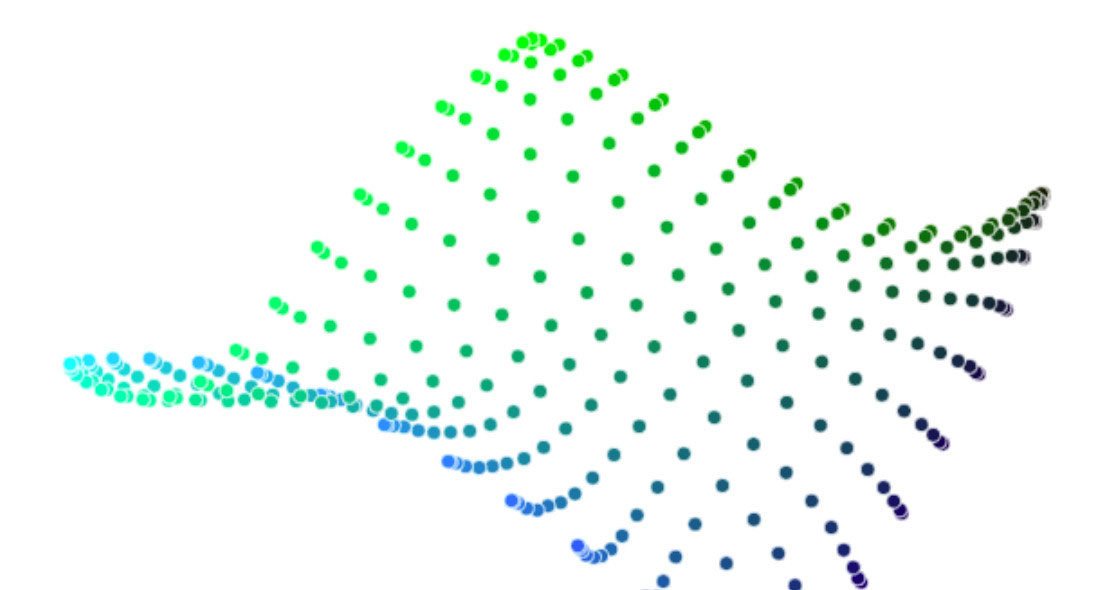
If you see a t-SNE plot with strange “pinched” shapes, chances are the process was stopped too early. Out of sight from the user, the algorithm makes all sorts of adjustments that tidy up its visualizations.

How to Use t-SNE Effectively
Although extremely useful for visualizing high-dimensional data, t-SNE plots can sometimes be mysterious or misleading.
https://distill.pub/2016/misread-tsne/

Visualizing Data using t-SNE
We present a new technique called "t-SNE" that visualizes
high-dimensional data by giving each datapoint a location in a two or
three-dimensional map. The technique is a variation of Stochastic
Neighbor Embedding (Hinton and Roweis, 2002) that is much easier to optimize,
and produces significantly better visualizations by reducing the
tendency to crowd points together in the center of the map. t-SNE is
better than existing techniques at creating a single map that reveals
structure at many different scales. This is particularly important for
high-dimensional data that lie on several different, but related,
low-dimensional manifolds, such as images ofobjects from multiple
classes seen from multiple viewpoints. For visualizing the structure
of very large data sets, we show how t-SNE can use random walks on
neighborhood graphs to allow the implicit structure of all of the data
to influence the way in which a subset of the data is displayed. We
illustrate the performance of t-SNE on a wide variety of data sets and
compare it with many other non-parametric visualization techniques,
including Sammon mapping, Isomap, and Locally Linear Embedding. The
visualizations produced by t-SNE are significantly better than those
produced by the other techniques on almost all of the data sets.
https://jmlr.org/papers/v9/vandermaaten08a.html

 Seonglae Cho