Diffusion Model

Diffusion Probabilistic model (DPM), Variational Diffusion Model

Diffusion models progressively add Gaussian noise to data (forward process) and learn to reverse this process step-by-step (reverse process). At high noise levels, the model recovers coarse, low-frequency structure; as noise decreases, it progressively refines the sample by adding higher-frequency details.

Diffusion models generate images by adding noise and then reversing it. Since white noise has energy across all frequencies but natural images have most energy in low frequencies, high-frequency components lose signal-to-noise ratio (SNR) first, making them harder to recover at early denoising steps.

Gradually add Gaussian noise with

Markov Chain to model increasing noise process. Generate images by sampling from Gaussian noise. After that, the model learns to reverse noise into images by denoising process with modeling noise distribution. Due to Explicit likelihood Modeling, it solves the drawback of

GAN where it covers less of the generation space.

Network Architecture

UNet like CNN image to image model is used as the reverse denoiser, often with

Attention Mechanism during later compression/decompression stages such as

Cross-Attention and image patches. Diffusion uses

Positional Embedding for each time step. which prevents effective extrapolation like transformer do not.

Integral

The statement "denoising = integration" refers to the continuous-time perspective, where diffusion/flow-based generation is formalized as following the solution of a differential equation that continuously moves the state from noise to data. Rather than "removing noise all at once," it involves accumulating "small denoising actions" tens to thousands of times (through integral approximation) to create the final image.

Classic

DDPM is a "discrete-time"

Markov Chain that repeats denoising steps (step-by-step updates rather than integration), but from a continuous-time perspective, it ultimately connects to numerically solving the reverse

SDE.

DDIM / probability-flow ODE / flow matching / rectified flow approaches explicitly take the form of directly integrating an ODE from the start.

Diffusion Model Notion

Diffusion Model Usages

Stable Diffusion WebUI

Fooocus

lllyasviel • Updated 2026 Jan 7 12:13

Diffusion Fine Tuning

SparseCtrl

Animate Anyone

CFG Scale

Distribution Matching Distillation

Diffusion Models

https://arxiv.org/pdf/2006.11239

arxiv.org

https://arxiv.org/pdf/2105.05233

Tutorial

arxiv.org

https://arxiv.org/pdf/2403.18103

smalldiffusion
yuanchenyang • Updated 2026 Jan 23 3:42

Through noise prediction, we can mathematically prove that the denoiser can be viewed as an "approximate projection" onto the data manifold, equivalent to the gradient of a smoothed distance function (

Moreau envelope). Gradient of a smoothed distance function to the manifold is equivalent as denoiser output, as a metaphor, trained denoiser generates force vectors that gradually bend towards the data manifold.

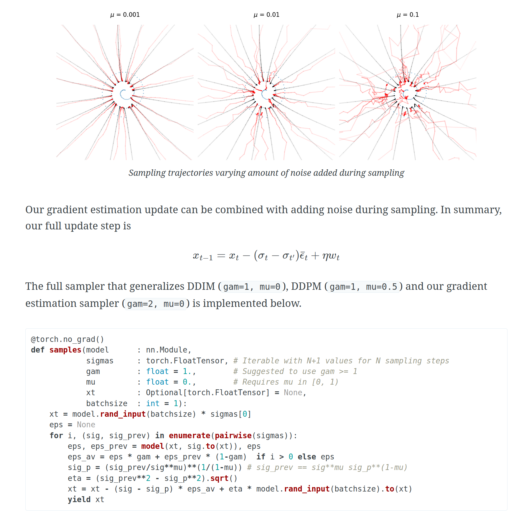
Then,

DDIM can be interpreted as gradient descent, combining momentum and

DDPM pddtechniques to improve convergence speed and image quality.

Diffusion models from scratch

This tutorial aims to give a gentle introduction to diffusion models, with a running example to illustrate how to build, train and sample from a simple diffusion model from scratch.